SymPy

SymPy (http://www.sympy.org/) is a Python module for symbolic mathematics. It’s similiar to commercial computer algebra systems like Maple or Mathematica.

Usage

Web service

SymPy live http://live.sympy.org/

SymPy gamma http://sympygamma.com/

Python Module

SymPy can be installed, imported and used like any other regular Python module.

Output can be done as nicely formatted LaTeX. This is a great way to get more complicated formulae into your manuscript insted of hassling with nested LaTeX commands. Right click on the outputted formula in any ipython notebook or the above mentioned web services to extract the corresponding LaTeX commands.

Basic Examples

%matplotlib inline
from sympy import *
Value error parsing header in AFM: b'UnderlinePosition' b'-133rUnderlineThickness 20rVersion 7.000'

init_printing() activates nicely formatted LaTeX output within an ipython notebook.

init_printing()

Symbols

Mathematical variables have to be defined as symbols before usage

x = Symbol('x')
type(x)
sympy.core.symbol.Symbol
(pi + x)**2
\[\left(x + \pi\right)^{2}\]

A short form of Symbol is S. Both can be used to define serveral symbols at once.

x,y,z = S('x,y,z')
x**2+y**2+z**2
\[x^{2} + y^{2} + z^{2}\]

Fractions

Fractions of nubers must be defined with Rational. Otherwise the numbers will be evaluated as a Python expression resulting in a regular Python floating point number.

4/7 # regular python division
\[0.5714285714285714\]
r1 = Rational(4,7) # sympy rational
r1
\[\frac{4}{7}\]
r2 = x/y # since x and y are already sympy symbols no explicit Rational definition is required
r2
\[\frac{x}{y}\]
r1*r2+1
\[\frac{4 x}{7 y} + 1\]

Complex Numbers

The imaginary unit is noted as I in sympy.

1+I
\[1 + i\]
I**2
\[-1\]
simplify((1+I)**2)
\[2 i\]

Numeric evaluation

r1.evalf(100)
\[0.5714285714285714285714285714285714285714285714285714285714285714285714285714285714285714285714285714\]
pi.evalf(100)
\[3.141592653589793238462643383279502884197169399375105820974944592307816406286208998628034825342117068\]

Substitution

f1 = x**2+x**3

subs can be used to evaluate a function at a specific point

f1.subs(x, 2)
\[12\]

or to substitute expressions

a=S('a')
f1.subs(x, a)
\[a^{3} + a^{2}\]
f2 = f1.subs(x, sqrt(a))
f2
\[a^{\frac{3}{2}} + a\]
f2.subs(a, 1)
\[2\]

Plotting

from sympy.plotting import plot
f1
\[x^{3} + x^{2}\]
plot(f1)
_images/8_sympy_37_0.png
<sympy.plotting.plot.Plot at 0x7f1b3125a5f8>
plot(f1, (x,-5,5))
_images/8_sympy_38_0.png
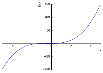
<sympy.plotting.plot.Plot at 0x7f1b11812e48>
f2
\[a^{\frac{3}{2}} + a\]
plot( f2)
_images/8_sympy_40_0.png
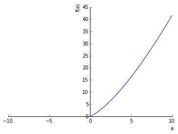
<sympy.plotting.plot.Plot at 0x7f1b117e2898>

Simplification

x,y=S('x,y')
eq = (x**3 + x**2 - x - 1)/(x**2 + 2*x + 1)
eq
\[\frac{x^{3} + x^{2} - x - 1}{x^{2} + 2 x + 1}\]
simplify(eq)
\[x - 1\]
simplify(sin(x)**2 + cos(x)**2)
\[1\]

Solving equations

x = S('x')
eq = x**2 - 1
eq
\[x^{2} - 1\]
plot(eq, (x, -2, +2))
_images/8_sympy_47_0.png
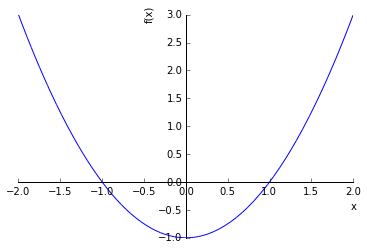
<sympy.plotting.plot.Plot at 0x7f1b117665f8>
solve(eq, x)
\[\left [ -1, \quad 1\right ]\]
eq = 2*x*y + y**2/2
solve(eq, y)
\[\left [ 0, \quad - 4 x\right ]\]

Differentiate

diff(2*x*y + y**2/2, y)
\[2 x + y\]

Integrate

integrate(2*x*y + y**2/2, y)
\[x y^{2} + \frac{y^{3}}{6}\]

Matrices

unity matrix

eye(10)
\[\begin{split}\left[\begin{matrix}1 & 0 & 0 & 0 & 0 & 0 & 0 & 0 & 0 & 0\\0 & 1 & 0 & 0 & 0 & 0 & 0 & 0 & 0 & 0\\0 & 0 & 1 & 0 & 0 & 0 & 0 & 0 & 0 & 0\\0 & 0 & 0 & 1 & 0 & 0 & 0 & 0 & 0 & 0\\0 & 0 & 0 & 0 & 1 & 0 & 0 & 0 & 0 & 0\\0 & 0 & 0 & 0 & 0 & 1 & 0 & 0 & 0 & 0\\0 & 0 & 0 & 0 & 0 & 0 & 1 & 0 & 0 & 0\\0 & 0 & 0 & 0 & 0 & 0 & 0 & 1 & 0 & 0\\0 & 0 & 0 & 0 & 0 & 0 & 0 & 0 & 1 & 0\\0 & 0 & 0 & 0 & 0 & 0 & 0 & 0 & 0 & 1\end{matrix}\right]\end{split}\]
m11, m12, m21, m22 = symbols("m11, m12, m21, m22")
b1, b2 = symbols("b1, b2")
A = Matrix([[m11, m12],[m21, m22]])
A
\[\begin{split}\left[\begin{matrix}m_{11} & m_{12}\\m_{21} & m_{22}\end{matrix}\right]\end{split}\]
b = Matrix([[b1], [b2]])
b
\[\begin{split}\left[\begin{matrix}b_{1}\\b_{2}\end{matrix}\right]\end{split}\]
A**2
\[\begin{split}\left[\begin{matrix}m_{11}^{2} + m_{12} m_{21} & m_{11} m_{12} + m_{12} m_{22}\\m_{11} m_{21} + m_{21} m_{22} & m_{12} m_{21} + m_{22}^{2}\end{matrix}\right]\end{split}\]
A * b
\[\begin{split}\left[\begin{matrix}b_{1} m_{11} + b_{2} m_{12}\\b_{1} m_{21} + b_{2} m_{22}\end{matrix}\right]\end{split}\]
A.det()
\[m_{11} m_{22} - m_{12} m_{21}\]
A.inv()
\[\begin{split}\left[\begin{matrix}\frac{1}{m_{11}} + \frac{m_{12} m_{21}}{m_{11}^{2} \left(m_{22} - \frac{m_{12} m_{21}}{m_{11}}\right)} & - \frac{m_{12}}{m_{11} \left(m_{22} - \frac{m_{12} m_{21}}{m_{11}}\right)}\\- \frac{m_{21}}{m_{11} \left(m_{22} - \frac{m_{12} m_{21}}{m_{11}}\right)} & \frac{1}{m_{22} - \frac{m_{12} m_{21}}{m_{11}}}\end{matrix}\right]\end{split}\]

Example: Calculate determinant of matrices in a loop

from IPython.display import display

#b01a01
A = Matrix( [[2,2,-5],[5,4,1],[4,14,3]]) # assign matrix to variable A
B = Matrix( [[1,2,3],[0,4,5],[0,0,6]]) # assign matrix to variable B
C = Matrix( [[1,2,-1,2],[-3,5,-5,-2],[5,4,3,-4], [-4,-3,5,5]]) # assign matrix to variable C

# show the result for each matrix
for M in (A, B, C):
    print( 'The determinant of matrix')
    display(M)
    print(' is ')
    display(M.det())
The determinant of matrix
\[\begin{split}\left[\begin{matrix}2 & 2 & -5\\5 & 4 & 1\\4 & 14 & 3\end{matrix}\right]\end{split}\]
is
\[-296\]
The determinant of matrix
\[\begin{split}\left[\begin{matrix}1 & 2 & 3\\0 & 4 & 5\\0 & 0 & 6\end{matrix}\right]\end{split}\]
is
\[24\]
The determinant of matrix
\[\begin{split}\left[\begin{matrix}1 & 2 & -1 & 2\\-3 & 5 & -5 & -2\\5 & 4 & 3 & -4\\-4 & -3 & 5 & 5\end{matrix}\right]\end{split}\]
is
\[1050\]

Example: Calculate Eigenvalues and Eigenvectors

a,b,c,d = S('a,b,c,d')
A = Matrix( [[a,b], [c,d]])
A
\[\begin{split}\left[\begin{matrix}a & b\\c & d\end{matrix}\right]\end{split}\]
A.eigenvals()
\[\left \{ \frac{a}{2} + \frac{d}{2} - \frac{1}{2} \sqrt{a^{2} - 2 a d + 4 b c + d^{2}} : 1, \quad \frac{a}{2} + \frac{d}{2} + \frac{1}{2} \sqrt{a^{2} - 2 a d + 4 b c + d^{2}} : 1\right \}\]
A.eigenvects()
\[\begin{split}\left [ \left ( \frac{a}{2} + \frac{d}{2} - \frac{1}{2} \sqrt{a^{2} - 2 a d + 4 b c + d^{2}}, \quad 1, \quad \left [ \left[\begin{matrix}- \frac{b}{\frac{a}{2} - \frac{d}{2} + \frac{1}{2} \sqrt{a^{2} - 2 a d + 4 b c + d^{2}}}\\1\end{matrix}\right]\right ]\right ), \quad \left ( \frac{a}{2} + \frac{d}{2} + \frac{1}{2} \sqrt{a^{2} - 2 a d + 4 b c + d^{2}}, \quad 1, \quad \left [ \left[\begin{matrix}- \frac{b}{\frac{a}{2} - \frac{d}{2} - \frac{1}{2} \sqrt{a^{2} - 2 a d + 4 b c + d^{2}}}\\1\end{matrix}\right]\right ]\right )\right ]\end{split}\]
B = A.subs(((a,1),(d,1)))
B
\[\begin{split}\left[\begin{matrix}1 & b\\c & 1\end{matrix}\right]\end{split}\]
B.eigenvals()
\[\left \{ - \sqrt{b c} + 1 : 1, \quad \sqrt{b c} + 1 : 1\right \}\]
B.eigenvects()
\[\begin{split}\left [ \left ( - \sqrt{b c} + 1, \quad 1, \quad \left [ \left[\begin{matrix}- \frac{b}{\sqrt{b c}}\\1\end{matrix}\right]\right ]\right ), \quad \left ( \sqrt{b c} + 1, \quad 1, \quad \left [ \left[\begin{matrix}\frac{b}{\sqrt{b c}}\\1\end{matrix}\right]\right ]\right )\right ]\end{split}\]