# this ipython magic command imports pylab and allows the plots to reside within the notebook
%pylab inline

Populating the interactive namespace from numpy and matplotlib

The following examples are based on Florian Lhuillier’s lecture on Matlab which can be found online:

http://geophysik.uni-muenchen.de/~lhuillier/teaching/AD2010/

Pylab continued …¶

Examples based on “… des données sous MATLAB”¶

set_printoptions(precision=2, suppress=True)

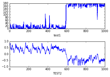
Excercise 1¶

aa = loadtxt('dipole_ref.txt')

aa.shape

(21481, 3)

subplot(211)
plot(aa[:,0], aa[:,1])
xlabel("test1")
subplot(212)
plot(aa[:,0], aa[:,2])
xlabel('TEST2')
subplots_adjust(hspace=.5)

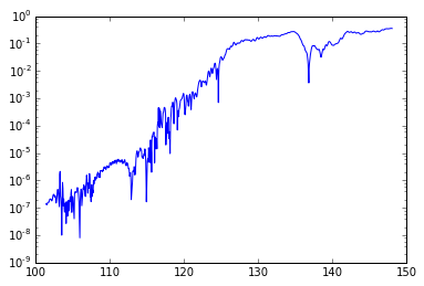
Excercise 2¶

aa = loadtxt('dipole_ref.txt')

bb = loadtxt('dipole_pert.txt')

t = bb[:,0];

d = bb[:,2] - interp(t, aa[:,0],aa[:,2]);

semilogy(t, abs(d))

[<matplotlib.lines.Line2D at 0x7f911be2add8>]

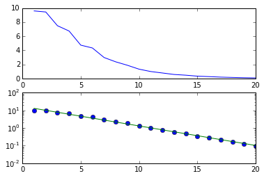
Excercise 3¶

d = genfromtxt('spectre.txt', skip_header=1, dtype=None, names=('name', 'number', 'amplitude'))

array([(b'a', 1, 9.5960921), (b'b', 2, 9.4450301), (b'c', 3, 7.5000147),
       (b'd', 4, 6.7446755), (b'e', 5, 4.7442346), (b'f', 6, 4.3416987),
       (b'g', 7, 2.9904522), (b'h', 8, 2.3769902), (b'i', 9, 1.8908512),
       (b'j', 10, 1.3387981), (b'k', 11, 1.0044059),
       (b'l', 12, 0.79748122), (b'm', 13, 0.5872564),
       (b'n', 14, 0.48502449), (b'p', 15, 0.34799267),
       (b'q', 16, 0.28167023), (b'r', 17, 0.20974501),
       (b's', 18, 0.16570928), (b't', 19, 0.12762576),
       (b'u', 20, 0.098378887)],
      dtype=[('name', 'S1'), ('number', '<i8'), ('amplitude', '<f8')])

Y=log(d['amplitude']); Y

array([ 2.26,  2.25,  2.01,  1.91,  1.56,  1.47,  1.1 ,  0.87,  0.64,
        0.29,  0.  , -0.23, -0.53, -0.72, -1.06, -1.27, -1.56, -1.8 ,
       -2.06, -2.32])

X = array((d['number'], 0*d['number']+1)).T; X

array([[ 1,  1],
       [ 2,  1],
       [ 3,  1],
       [ 4,  1],
       [ 5,  1],
       [ 6,  1],
       [ 7,  1],
       [ 8,  1],
       [ 9,  1],
       [10,  1],
       [11,  1],
       [12,  1],
       [13,  1],
       [14,  1],
       [15,  1],
       [16,  1],
       [17,  1],
       [18,  1],
       [19,  1],
       [20,  1]])

X.shape, Y.shape

((20, 2), (20,))

A = lstsq(X, Y)[0]; A

array([-0.25,  2.82])

subplot(211)
plot(d['number'], d['amplitude'])
subplot(212)
semilogy(d['number'], d['amplitude'], 'o')
semilogy(d['number'], exp(X.dot(A)))

[<matplotlib.lines.Line2D at 0x7f9119b37ac8>]

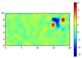
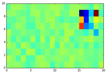
Excercise 4¶

aa = loadtxt('anomalie.txt')

nx = len( unique(aa[:,0])); nx

ny = len( unique(aa[:,1])); ny

X=aa[:,0].reshape((nx, ny));

Y=aa[:,1].reshape((nx, ny));

data = aa[:,2].reshape((nx, ny));

pcolor( X, Y, data)

<matplotlib.collections.PolyCollection at 0x7f9119cbe278>

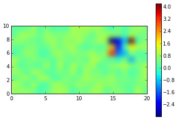
imshow(data.T,
           extent=[X.min(), X.max(), Y.min(), Y.max()],
           interpolation='gaussian', origin='lower')
colorbar()

<matplotlib.colorbar.Colorbar at 0x7f9119b30ef0>

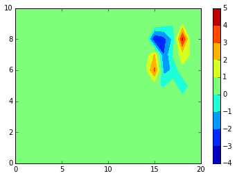
contourf( X, Y, data)
colorbar()

<matplotlib.colorbar.Colorbar at 0x7f9119d93470>

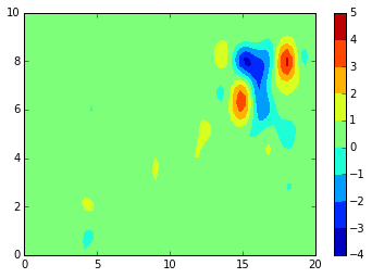
from scipy.ndimage import zoom

data = array(zoom(data,3)).T

contourf(data, extent=[X.min(), X.max(), Y.min(), Y.max()])
colorbar()
#axis("equal")

<matplotlib.colorbar.Colorbar at 0x7f9116fb7be0>

imshow(data,
           extent=[X.min(), X.max(), Y.min(), Y.max()],
           interpolation='gaussian', origin='lower', aspect=1)
colorbar()

<matplotlib.colorbar.Colorbar at 0x7f9116ef5240>